Rotating Hexominoes
by kbob
[This post is auto-generated from a Jupyter notebook]
Rotating Hexominoes
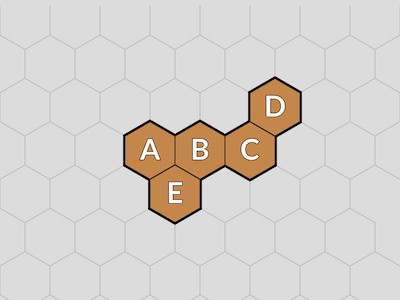
Suppose you have a hexomino on a grid. (Figure 1.)
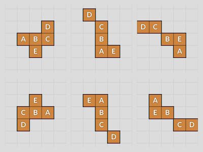
Because computers like rectangles better than hexes, let's map it to a square grid by skewing it . (Figure 2.) Each row is skewed half a unit left of the row below.

Computer is happy with that.
But now, you want to rotate your hexomino within the grid. On the hex grid, it's straightforward to set up a rotation matrix and transform the tile. The rotation matrix looks like this.
$$ (x', y') = \begin{bmatrix} cos \theta & -sin \theta \\ sin \theta & cos \theta \end{bmatrix} \begin{bmatrix} x \\ y \end{bmatrix} $$
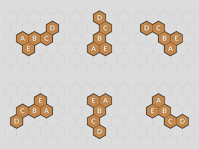
There are six possible rotations. See Figure 3.
This notebook is about how to rotate the hexomino in a rectangular grid.
from collections import namedtuple
from math import pi
import numpy as np

a = pi/3
c, s = cos(a), sin(a)

x = np.array([1.0, 0.0])
y = np.array([0.0, 1.0])
m = np.matmul
ac = np.allclose

X = '\N{MULTIPLICATION X}'
SN1 = '\N{SUPERSCRIPT MINUS}\N{SUPERSCRIPT ONE}'
We're going to start with a tile's location in rectangular coordinates, $ (x, y) $. Then we'll warp it into its hex coordinate location, rotate it, and warp it back.
Skew
First, skew. As mentioned, The rectangular coordinates have a leftward skew. So create a skew matrix to undo that.
$$ Skew = \begin{bmatrix} 1 && 1/2 \\ 0 && 1 \end{bmatrix} $$
While we're here, we'll calculate the inverse skew matrix to return to rectangular coordintes.
$$ Skew^{-1} = \begin{bmatrix} 1 && -1/2 \\ 0 && 1 \end{bmatrix} $$
# Skew right by pi/6
skew = np.array([[1, c], [0, 1]])
iskew = np.linalg.inv(skew)

print('Skew')
print(f'  x -> {m(skew, x)}')
print(f'  y -> {m(skew, y)}')
print()
print(f'Skew{SN1}')
print(f'  x -> {m(iskew, x)}')
print(f'  y -> {m(iskew, y)}')

assert ac(m(skew, x), [1, 0])
assert ac(m(skew, y), [0.5, 1])
assert ac(m(iskew, x), [1, 0])
assert ac(m(iskew, y), [-0.5, 1])
assert ac(m(iskew, m(skew, x)), x)
Skew
  x -> [1. 0.]
  y -> [0.5 1. ]

Skew⁻¹
  x -> [1. 0.]
  y -> [-0.5  1. ]
Scale
That didn't quite work. Hex tiles are further apart in the horizontal direction than in the vertical. So we can apply an anisotropic scale to shrink the Y coordinate. $ s $ is the height of a unit equilateral triangle, $ \sqrt{3} / 2 $.
$$ Scale = \begin{bmatrix} 1 & 0 \\ 0 & s \end{bmatrix} $$
Again, we'll calculate the inverse scale transform to map back to rectangular.
$$ Scale^{-1} = \begin{bmatrix} 1 & 0 \\ 0 & 1/s \end{bmatrix} $$
# Scale in Y

scale = np.array([[1, 0], [0, s]])
iscale = np.linalg.inv(scale)

print('Scale')
print(f'  x -> {m(x, scale)}')
print(f'  y -> {m(y, scale)}')
print()
print(f'Scale{SN1}')
print(f'  x -> {m(x, iscale)}')
print(f'  y -> {m(y, iscale)}')

assert ac(m(x, scale), x)
assert ac(m(y, scale), [0, s])
assert ac(m(x, iscale), x)
assert ac(m(y, iscale), [0, 1/s])
Scale
  x -> [1. 0.]
  y -> [0.        0.8660254]

Scale⁻¹
  x -> [1. 0.]
  y -> [0.         1.15470054]
Test that those two work together. Scale ✕ Skew. (We apply transforms right-to-left, as is the graphics way. I don't know why.)
# Skew and Scale

# print(f'Skew {X} Scale')
# print(f'  x -> {m(m(scale, skew), x)}')
# print(f'  y -> {m(m(scale, skew), y)}')

for xform in [m(scale, skew)]:
    print(f'Scale {X} Skew')
    print(f'  x -> {m(xform, x)}')
    print(f'  y -> {m(xform, y)}')
    assert ac(m(xform, x), x)
    assert ac(m(xform, y), [c, s])
Scale ✕ Skew
  x -> [1. 0.]
  y -> [0.5       0.8660254]
Rotation
Here's the rotation matrix. We only need rotation by $ \frac{pi}{3} $; we can get other rotations by repeating this rotation.
$$ s = sin \frac{pi}{3} = \frac{\sqrt{3}}{2} $$ $$ c = cos \frac{pi}{3} = \frac{1}{2} $$ $$ Rotation = \begin{bmatrix} c & -s \\ s & c \end{bmatrix} $$
# Rotate by pi/3

rotate = np.array([[c, -s], [s, c]])

print('Rotate')
print(f'  x -> {m(rotate, x)}')
print(f'  y -> {m(rotate, y)}')

assert ac(m(rotate, x), [c, s])
assert ac(m(rotate, y), [-s, c])
Rotate
  x -> [0.5       0.8660254]
  y -> [-0.8660254  0.5      ]
Test that all three work. Rotate ✕ Scale ✕ Skew.
# Skew, Scale, and Rotate

for xform in [m(m(rotate, scale), skew)]:
    print('Rotate {X} Scale {X} Skew')
    print(f'  x -> {m(xform, x)}')
    print(f'  y -> {m(xform, y)}')
    assert ac(m(xform, x), [c, s])
    assert ac(m(xform, y), [-c, s])
Rotate {X} Scale {X} Skew
  x -> [0.5       0.8660254]
  y -> [-0.5        0.8660254]
Now we can build and test the whole transform. Skew, scale, rotate, unscale, and unskew. Or in graphics convention, unskew ✕ unscale ✕ rotate ✕ scale ✕ skew.
# Skew, Scale, Rotate, Unscale, Unskew

for xform in [m(m(m(m(iskew, iscale), rotate), scale), skew)]:
    print(f'Skew{SN1} {X} Scale{SN1} {X} Rotate {X} Scale {X} Skew')
    print(f'xform = \n{xform}\n')
    print(f'  x -> {m(xform, x)}')
    print(f'  y -> {m(xform, y)}')
    assert ac(m(xform, x), [0, 1])
    assert ac(m(xform, y), [-1, 1])
Skew⁻¹ ✕ Scale⁻¹ ✕ Rotate ✕ Scale ✕ Skew
xform =
[[-2.33363804e-17 -1.00000000e+00]
 [ 1.00000000e+00  1.00000000e+00]]

  x -> [-2.33363804e-17  1.00000000e+00]
  y -> [-1.  1.]
The Transform
You'll note that our complete transform is dirty integers. (We love IEEE-754!) That's expected, because we want rotation to move tiles into actual cells, not the interstices between.
So the whole transform boiled down to this.
$$ Skew^{-1} × Scale^{-1} × Rotate × Scale × Skew = \begin{bmatrix} 0 & -1 \\ 1 & 1 \end{bmatrix} $$
# Build the transform.
#
# After all that, it's a really simple result.

xform = m(m(m(m(iskew, iscale), rotate), scale), skew)
assert ac(xform, np.rint(xform))
xform = np.rint(xform).astype('int')

print('Full Transform')
print(f'  [{xform[0, 0]:2} {xform[0, 1]:2}]')
print(f'  [{xform[1, 0]:2} {xform[1, 1]:2}]')
Full Transform
  [ 0 -1]
  [ 1  1]
Testing
Let's check the directions of the six neighbors.
tv = namedtuple('test_vector', 'input, expected')
tests = [
    tv([1, 0], [0, 1]),
    tv([0, 1], [-1, 1]),
    tv([-1, 1], [-1, 0]),
    tv([-1, 0], [0, -1]),
    tv([0, -1], [1, -1]),
    tv([1, -1], [1, 0]),
]

for t in tests:
    actual = m(xform, t.input)
    result = all(actual == t.expected)
    message = f'input {t.input}: expected {t.expected}, got {actual}'
    assert result, message

print('OK!')
OK!
That's it. Here's the example hexomino rotated through all six positions. (Figure 4.) But first, here's Figure 3 again for comparison.
Thanks for reading!